
Project #1: Assessing a CONUS-wide Synthetic Population of Forest Attributes
Beginning with my first project, my research team and I were tasked with determining if a KBAABB population is a good proxy for the true population of forest attributes, focusing on basal area, volume, count, biomass, and carbon. However, before diving head first into this project, it is essential that we have an understanding of what KBAABB is. Simply put, KBAABB is a synthetic population of the previously mentioned forest attributes created by using bootstrap-weighted sampling borrowing from kNN (k-Nearest-Neighbors).There were different types of KBAAB population each being, TNT(tree/no tree), Class(Vegetation class) and Subclass(Vegetation Subclass). All three of these KBAABB population where put up against actual FIA forest data to see whether or not any of these classes are a good proxy. The reason why KBABB was our main point of interest was due to having the potential to represent the true population of forests in the US while also being helpful in running simulations when the true population is required. So with this in mind, let’s focus on what I managed to accomplish on this project.
To assist in seeing if the KBAABB population is a good proxy for the true population of forest attributes, I decided to see whether or not each KBAABB population was over-borrowing from non-forest areas. To test this question, I decided to look at summary statistics of the Basal Area variable for each KBAABB population and compare them to the original FIA Basal Area variable. To not get overwhelmed by the amount of data, I subsectioned down to only looking at counties in the state of Arizona.
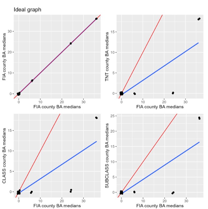
The first summary statistic I looked at was the median for Basal Areal. In the figure above the red line represents the xy line (Perfect Alignment) while the blue line represents the LSR line (Estimated Regression Line). The main thing we want to see from this figure above is the xy and LSR line to fall closely on each other to show how each KBAABB method relates to the FIA data. Further analyzing this figure gives us the main takeaways being that compared to our ideal graph, each KBAABB method has a LSR line lower than the xy line. Additionally, the medians in the KBAABB basal area data sets include many more values of zero for each county compared to FIA. With this in mind, this raised an eyebrow as the KBAABB population having inflated zeroes than the FIA data could mean that it is borrowing from not so great areas. I decided to look more closely at the zero proportions for Basal Area to get a better sense why this is the case.
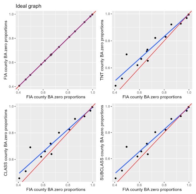
Before addressing the zero proportions one might ask why does the FIA data even have zeros? Well the answer to this is simple; there are Arizona Counties with no Basal Area. This logically makes sense as Arizona is mostly a dry barren state with a lack of greenery. Now with this in mind, to confirm the presence of inflated zeros, each KBAABB population was up against the FIA population to identify the zero proportions for Basal Area. The figure above shows that each KBAABB population had an estimated regression line very slightly above that xy line.Specifically, when examining each KBAABB estimated regression line, they all appear to perform similarly as each population looks to over-inflate the number of zeros. Though out of all populations. the best performing KBAABB population is the Subclass synthetic population, as it has a slope closer to the X-Y line.
With the results from our zero proportion looking to over inflate the number of zeroes within each KBAABB population, it brought to light an important question of whether or KBAABB produces distributions of forests that reflect reality. To answer this question, I took initiative to look at the spacial correlation for each KBAABB population vs the FIA population data. To do so, I constructed a Variogram of the Above Ground Carbon variable for each KBAABB population and compared it to the FIA data. For this section rather than focusing on multiple counties within Arizona, I filtered down to only one county to analyze specifically how each KBAABB populations spacial correlation would related to the true FIA data.
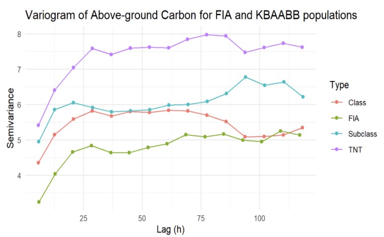
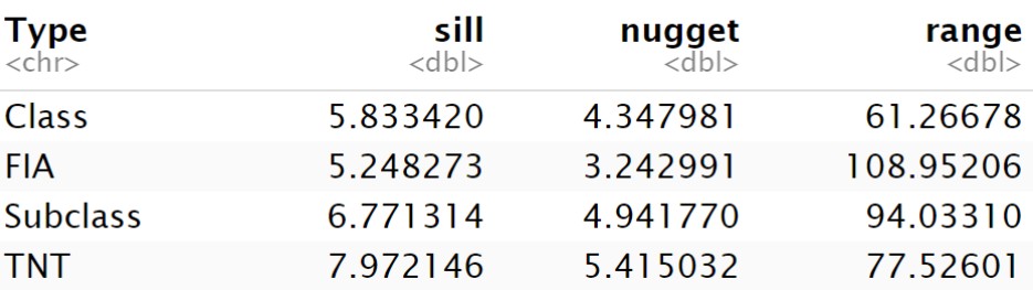
Before digging into what this figure above is displaying to us about Spacial Correlation, we need to know the In’s and Out’s of how a Variogram works. To begin with, let’s looks at the two axis. The X-axis represents the distance or lag between sample points in our data while the Y-axis represents the dissimilarity between data points at different spatial locations or the semivariance. Looking more closely at the numeric data below the figure introduces us to the Sill,Range and Nugget. All three of these components are important as they all illustrate where Spatial correlation is no longer present with noise. With these values in mind we are able to compare each KBAABB population to the true FIA data by following the three criteria for what we want to see in a Variogram.That criteria being a Low nugget (low measurement noise), Low sill (lower total variability) and a High range (spatial autocorrelation extends farther). Now when looking at the three KBAABB population up against each other, the KBAABB Class Population goes two for three on all criteria resulting in this population performing the best for spacial correlation compared the true FIA data and generally keeping spatial patterns and key relationships preserved.
Project #2: A Differentially Private Version of FIA Data
Before fully jumping into my second project, it’s crucial to provide a back to why my group and I focused on differential privacy. When looking into how the FIA routinely privatizes data, their method consists of randomly jittering and swapping the coordinates of its plots and coordinates. However, this method know as Fuzzing-and-Swapping suffers from two potential issues. The first issue of Fuzzing-and-Swapping is that it lacks a consistent way for measuring its own level of privacy protection and the second issue is that it significantly reduces the accuracy of small area estimates,rendering useless estimates for small areas containing few FIA plots. With these two major flaws in mind, my group and I looked into the “potential successor” to Fuzz-and-Swap that being Differential Privacy. Differential privacy can be defined as a mathematical framework that provides a strong, quantifiable guarantee of individual privacy when analyzing a data set. It works by ensuring that the output of a data analysis is nearly identical, regardless of whether any single individual’s data is included or excluded from the data set. This is achieved by introducing carefully calibrated statistical noise, controlled by a “privacy budget” (epsilon, ε), making it impossible for a harmful outside party with auxiliary information to learn specific details about any one person. With the introduction out of the way, let’s dive into this project. When translating the findings from numerous research papers on differential privacy into an R project, several packages were available to facilitate this process. The main R package that we’ve been experimenting with is diffpriv. The package allows us to implement the formal framework of differential privacy in an automated process. For example, it contains generic mechanisms for privatizing non-private target functions, such as the Laplace, Gaussian, exponential, and Bernstein mechanisms, as well as a way to estimate sensitivity for non-private targets, which removes the need for additional mathematical analysis for sensitivity bounds. When getting started with using the diffpriv package, we kept it simple to familiarize ourselves with the package by beginning with privatizing summary statistics for a singular variable in the FIA dataset. A new data frame was created with only the FIA Basal Area (labeled as “fia_BA”) to begin testing. After loading the diffpriv package, a target function was created to select what summary statistic would be privatized. Next, a Laplace mechanism was introduced to add Laplace noise to the output of the target function (in this case, the mean). From here, the next step was to set and calculate the sensitivity by determining the range of the fia_BA dataset and then dividing by the length of the dataset to scale the sensitivity for the mean function. Following this, it is necessary to inform R that the output of the target function is 1-dimensional so that the package can function properly. Finally, the last step is to privatize and print the response. This is done by setting our fia_BA equal to a vector x and using the releaseResponse() function to apply the differential privacy mechanism. Within this function, an additional function of DPParamsEps() defines the privacy budget of ε. The mechanism then finally outputs a privatized version of target(X), the mean of X with Laplace noise.
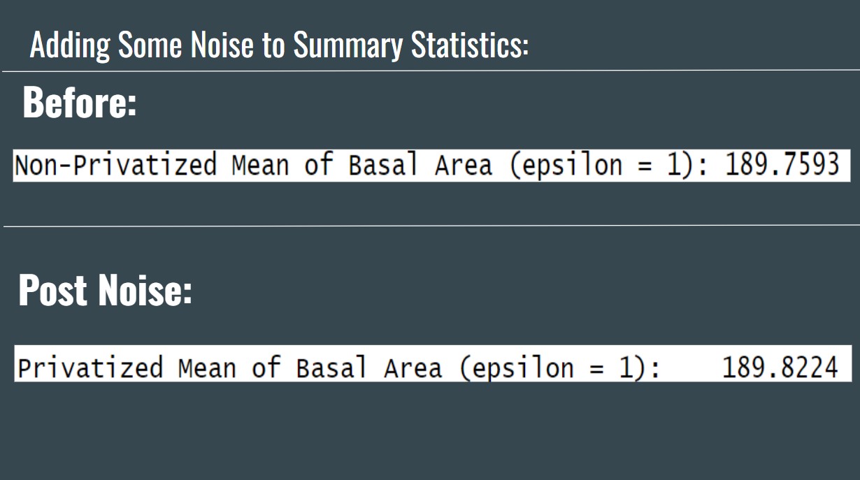
After getting familiar with the package, the next objective was to create a brand new dataset consisting of the privatization of an entire column for a variable. Even though this has been achieved, we have some questions on how the code specifically works and until figured out, will not be considered differentially private. However, with the code we have we were able to still create pseudo-privatized data of an Arizona counties Latitude and Longitude. The figure below illustrates how adjusting our epsilon value affects the distribution of scattered points for privatized data.
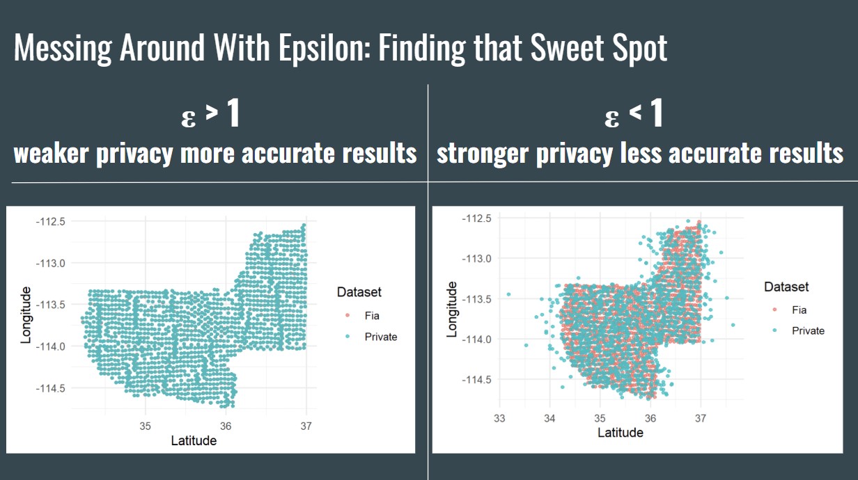
The figure above shows that when adjusting our ε value, when ε > 1 the weaker privacy but the more accurate results and when ε < 1 the stronger privacy but the less accurate results. This ends my project with two overarching big question for the future for differential privacy for FIA. Those being finding that special ε to obtain that perfect balance between data privacy and accurate results for meaningful analysis and quantifying whether or not our privatized data is accurate. Both questions serve as monumental task to finally achieving that sweet privacy and protection we seek within our own personal data.